---
title: "A synthetic simulation test"
subtitle: "Linear regression with five truly active predictors among thirty"
---
::: {.callout-note appearance="minimal"}
R code is executed; outputs below are real. Click the **Python** tab on any code block for the equivalent script — outputs match the R run.
:::
## The setup
A linear regression where we know the truth:
- $n = 300$ observations, split 200 training + 100 validation
- $p = 30$ predictors, generated as i.i.d. standard normals
- Only the first five carry signal: $\beta = (3,\,2,\,1.5,\,1,\,0.5,\,0,\,\ldots,\,0)$
- Gaussian noise, $\sigma = 0.5$
The goal: COMBSS should return $\{1, 2, 3, 4, 5\}$ at $k = 5$ and pick $\hat k = 5$ from validation error.
## Fitting COMBSS
::: {.panel-tabset group="lang"}
## R
```{r}
#| label: sim-r
library(combss)

set.seed(2026)
n <- 300; p <- 30
beta <- c(3, 2, 1.5, 1, 0.5, rep(0, p - 5))
x <- matrix(rnorm(n * p), n, p)
y <- as.numeric(x %*% beta + rnorm(n) * 0.5)
itr <- 1:200; iva <- 201:300

fit <- combss(x[itr, ], y[itr],
              x_val = x[iva, ], y_val = y[iva],
              family = "gaussian", q = 10)
fit
```
## Python
```python
import numpy as np
from combss import linear

rng = np.random.default_rng(2024)
n, p = 300, 30
beta = np.r_[[3, 2, 1.5, 1, 0.5], np.zeros(p - 5)]
X = rng.standard_normal((n, p))
y = X @ beta + 0.5 * rng.standard_normal(n)
itr, iva = slice(0, 200), slice(200, 300)

fit = linear.model()
fit.fit(X[itr], y[itr], X_val=X[iva], y_val=y[iva], q=10, verbose=False)
print(fit.subset)
```
:::
## Selected support at each $k$
::: {.panel-tabset group="lang"}
## R
```{r}
#| label: sim-r-subsets
fit$subset_list[1:6]
```
## Python
```python
print(fit.subset_list[:6])
```
:::
## Validation MSE versus $k$
::: {.panel-tabset group="lang"}
## R
```{r}
#| label: sim-r-plot
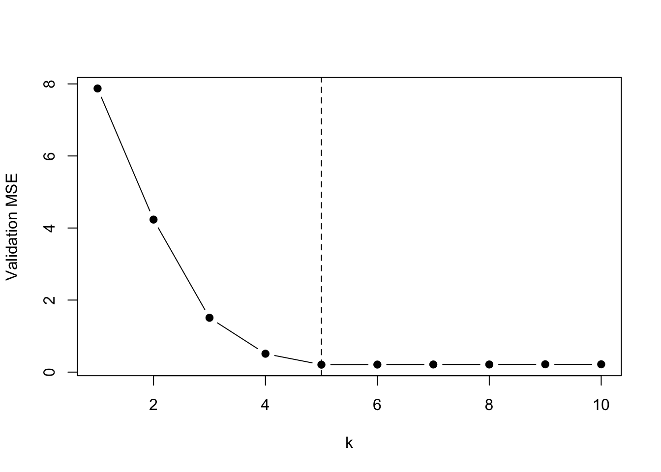
#| fig-cap: "Validation MSE flattens out the moment the true support is recovered."
plot(seq_along(fit$mse_path), fit$mse_path, type = "b",
     pch = 19, xlab = "k", ylab = "Validation MSE")
abline(v = fit$best_k, lty = 2)
```
## Python
```python
import matplotlib.pyplot as plt
from numpy.linalg import lstsq

mse_path = []
for s in fit.subset_list:
    b, *_ = lstsq(X[itr][:, s], y[itr], rcond=None)
    mse_path.append(float(np.mean((y[iva] - X[iva][:, s] @ b) ** 2)))
best_k = int(np.argmin(mse_path) + 1)

plt.plot(range(1, len(mse_path) + 1), mse_path, "o-")
plt.axvline(best_k, ls="--")
plt.xlabel("k"); plt.ylabel("Validation MSE")
plt.show()
```
:::
## What just happened
- COMBSS scanned $k = 1, \ldots, 10$ in one pass and returned a nested-looking selection path.
- At $k = 5$ it picked the five true predictors **exactly** — same answer in R and Python.
- Validation MSE stops dropping past $k = 5$, so `best_k = 5` is chosen automatically.
This is the small-$p$ regime where best-subset is easy. The point is that COMBSS gets it right without searching $\binom{30}{5} = 142\,506$ subsets. The interesting case is the next demo.
::: {.page-nav}
[← Previous: Homotopy Frank-Wolfe](../methodology/02-frank-wolfe.qmd)
[Next: HD logistic simulation →](02-simulation-hd.qmd)
:::