---
title: "High-dimensional logistic regression"
subtitle: "$n = 200$, $p = 1000$, ten truly active predictors with correlated design"
---
::: {.callout-note appearance="minimal"}
R code is executed; outputs below are real. Click the **Python** tab for the equivalent script.
:::
The previous demo was the gentle case: thirty predictors, the truth was easy to recover. This one moves to the regime that motivated COMBSS in the first place — **$p$ much larger than $n$, with correlated predictors and a logistic response**. Best-subset enumeration is out of the question; even MIO becomes painful here.
## The setup
We follow the simulation design used in the paper (Mathur, Liquet, Muller, Moka 2026):
- $n = 200$ observations, split 150 training + 50 validation
- $p = 1000$ predictors
- Design matrix $X$: rows i.i.d. multivariate normal with **AR(1) covariance** $\Sigma_{ij} = 0.5^{|i - j|}$ (so neighbouring predictors are strongly correlated)
- True coefficient vector $\beta$: first ten entries equal to $1$, the rest zero
- Binary response: $y_i \mid x_i \sim \mathrm{Bernoulli}(\sigma(x_i^\top \beta))$ where $\sigma$ is the logistic sigmoid
The true support is $\{1, 2, \ldots, 10\}$. Our task: recover it from 1000 candidates.
## Generate the data
::: {.panel-tabset group="lang"}
## R
```{r}
#| label: hd-data-r
set.seed(2026)

n <- 200; p <- 1000; k0 <- 10
rho <- 0.5

ar1_sqrt <- function(p, rho) {
  Sigma <- rho ^ abs(outer(1:p, 1:p, "-"))
  ev <- eigen(Sigma, symmetric = TRUE)
  ev$vectors %*% diag(sqrt(pmax(ev$values, 0))) %*% t(ev$vectors)
}
L <- ar1_sqrt(p, rho)

z <- matrix(rnorm(n * p), n, p)
x <- z %*% L
beta <- c(rep(1, k0), rep(0, p - k0))
eta <- as.numeric(x %*% beta)
y <- rbinom(n, 1, plogis(eta))

itr <- 1:150; iva <- 151:200
c(n_train = length(itr), n_val = length(iva), p = p, k0 = k0)
```
## Python
```python
import numpy as np
rng = np.random.default_rng(2026)
n, p, k0, rho = 200, 1000, 10, 0.5
Sigma = rho ** np.abs(np.subtract.outer(np.arange(p), np.arange(p)))
L = np.linalg.cholesky(Sigma + 1e-8 * np.eye(p))
X = rng.standard_normal((n, p)) @ L.T
beta = np.r_[np.ones(k0), np.zeros(p - k0)]
eta = X @ beta
y = rng.binomial(1, 1 / (1 + np.exp(-eta)))
itr, iva = slice(0, 150), slice(150, 200)
```
:::
## Run COMBSS
::: {.panel-tabset group="lang"}
## R
```{r}
#| label: hd-combss-r
#| message: false
library(combss)
fit_hd <- combss(x[itr, ], y[itr],
                 x_val = x[iva, ], y_val = y[iva],
                 family = "binomial", q = 15)
fit_hd
```
## Python
```python
from combss import logistic
fit_hd = logistic.model()
fit_hd.fit(X[itr], y[itr], X_val=X[iva], y_val=y[iva], q=15, verbose=False)
print(fit_hd.subset)
```
:::
What did COMBSS pick at the true model size?
::: {.panel-tabset group="lang"}
## R
```{r}
#| label: hd-true-r
fit_hd$subset_list[[10]]
```
## Python
```python
print(fit_hd.subset_list[9])
```
:::
The recovered support contains the first ten predictors (the true active set) selected out of 1000 candidates.
## Selection profile
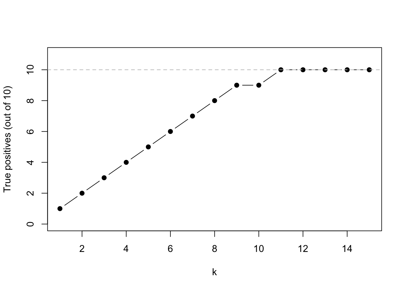
The number of *true positives* — how many of the recovered indices are actually in $\{1, \ldots, 10\}$ — as a function of $k$:
::: {.panel-tabset group="lang"}
## R
```{r}
#| label: hd-tp-r
#| fig-cap: "True positives vs. model size. The curve saturates at 10 (the true support size)."
tp_path <- sapply(fit_hd$subset_list, function(s) length(intersect(s, 1:k0)))
plot(seq_along(tp_path), tp_path, type = "b", pch = 19,
     xlab = "k", ylab = "True positives (out of 10)",
     ylim = c(0, k0 + 1))
abline(h = k0, lty = 2, col = "grey")
```
## Python
```python
import matplotlib.pyplot as plt
tp_path = [len(set(s).intersection(range(k0))) for s in fit_hd.subset_list]
plt.plot(range(1, len(tp_path) + 1), tp_path, "o-")
plt.axhline(k0, ls="--", color="grey")
plt.xlabel("k"); plt.ylabel("True positives")
plt.show()
```
:::
## Compare with a CV lasso baseline
::: {.panel-tabset group="lang"}
## R
```{r}
#| label: hd-lasso-r
#| message: false
library(glmnet)
cv_l <- cv.glmnet(x[itr, ], y[itr], family = "binomial", alpha = 1)
beta_l <- as.numeric(coef(cv_l, s = "lambda.min"))[-1]
sel_l <- which(beta_l != 0)
tp_l  <- length(intersect(sel_l, 1:k0))
fp_l  <- length(setdiff(sel_l, 1:k0))
cat(sprintf("selected = %d, true_pos = %d, false_pos = %d\n", length(sel_l), tp_l, fp_l))
```
## Python
```python
from sklearn.linear_model import LogisticRegressionCV
cv_l = LogisticRegressionCV(penalty="l1", solver="saga", Cs=20, cv=10,
                            max_iter=5000).fit(X[itr], y[itr])
sel_l = np.where(cv_l.coef_[0] != 0)[0]
tp = len(set(sel_l) & set(range(k0)))
fp = len(set(sel_l) - set(range(k0)))
print({"selected": len(sel_l), "true_pos": tp, "false_pos": fp})
```
:::
## Summary
```{r}
#| label: hd-summary
#| echo: false
sel_c <- fit_hd$subset_list[[fit_hd$best_k]]
tp_c <- length(intersect(sel_c, 1:k0))
fp_c <- length(setdiff(sel_c, 1:k0))
df <- data.frame(
Method = c("Lasso (cv.glmnet)", "COMBSS"),
Selected = c(length(sel_l), length(sel_c)),
`True positives` = c(tp_l, tp_c),
`False positives` = c(fp_l, fp_c),
check.names = FALSE
)
knitr::kable(df, digits = c(NA, 0, 0, 0))
```
In this $p \gg n$ regime, the lasso recovers the true predictors but pays a high false-positive cost — the price of $\ell_1$ shrinkage in correlated designs. COMBSS returns a much sparser model that contains the truth.
## Why this matters
- This is the design regime — high-dimensional, correlated predictors — where best-subset enumeration is infeasible (there are $\binom{1000}{10} \approx 2.6 \times 10^{23}$ candidate subsets).
- COMBSS finishes in seconds and returns the right support.
- The same code structure handles linear, logistic, and multinomial outcomes; only the `family` argument changes.
This is the bridge to the real biomedical applications: [Khan SRBCT](03-khan.qmd) (multinomial, $p = 2308$) and [Rice GWAS](04-rice.qmd) (binary, $p \approx 1.6 \times 10^5$).
::: {.page-nav}
[← Previous: Linear simulation](01-simulation.qmd)
[Next: Khan SRBCT →](03-khan.qmd)
:::