---
title: "COMBSS (our method)"
subtitle: "Where it sits between lasso and MIO"
---

## Where COMBSS fits

Three properties we want a method to have:

1. **Continuous / smooth optimisation** — tractable, gradient-based, scalable.
2. **Targets the $\ell_0$-constrained problem** — faithful to the original sparse selection task.
3. **Returns exactly $k$ features** — gives the user direct control over model size.

```{=html}
<div class="venn-wrap">
<svg viewBox="-40 -30 620 470" xmlns="http://www.w3.org/2000/svg" role="img" aria-label="Venn diagram showing COMBSS at the centre of three properties.">
  <circle cx="270" cy="120" r="125" fill="#2a9d8f" fill-opacity="0.22" stroke="#1f7a70" stroke-width="1.6"/>
  <circle cx="190" cy="230" r="125" fill="#e76f51" fill-opacity="0.22" stroke="#b04a31" stroke-width="1.6"/>
  <circle cx="350" cy="230" r="125" fill="#e9c46a" fill-opacity="0.28" stroke="#9c7d22" stroke-width="1.6"/>
  <text x="270" y="-12" font-size="18" font-weight="700" fill="#1f7a70" text-anchor="middle">Returns exactly k features</text>
  <text x="140" y="378" font-size="18" font-weight="700" fill="#b04a31" text-anchor="middle">Continuous /</text>
  <text x="140" y="400" font-size="18" font-weight="700" fill="#b04a31" text-anchor="middle">smooth optimisation</text>
  <text x="400" y="378" font-size="18" font-weight="700" fill="#9c7d22" text-anchor="middle">Targets ℓ₀-</text>
  <text x="400" y="400" font-size="18" font-weight="700" fill="#9c7d22" text-anchor="middle">constrained problem</text>
  <text x="130" y="290" font-size="19" font-style="italic" fill="#0b3a35" text-anchor="middle">Lasso</text>
  <text x="340" y="148" font-size="19" font-style="italic" fill="#0b3a35" text-anchor="middle">MIO</text>
  <text x="270" y="227" font-size="24" font-weight="700" fill="#0b3a35" text-anchor="middle">COMBSS</text>
</svg>
</div>
```

- **Lasso** sits only in the *smooth optimisation* circle — convex and scalable, but doesn't target $\ell_0$ and doesn't directly control $k$.
- **MIO** sits in *targets $\ell_0$* and *returns $k$* — exact but not a smooth optimisation, and not scalable.
- **COMBSS** sits in all three.

## The bridge: side by side

| | **Lasso** | **MIO** | **COMBSS** |
|---|---|---|---|
| Variable type | $\boldsymbol{\beta} \in \mathbb{R}^p$ | $\boldsymbol{s} \in \{0,1\}^p$ | $\boldsymbol{t} \in [0,1]^p$ |
| Sparsity by | $\ell_1$ penalty | hard $\ell_0$ + Big-$M$ | continuous relaxation on the support indicator |
| Selection size | indexed by $\lambda$ | $k$ via constraint | $k$ via polytope |
| Scales to $p \gg n$ | yes | barely | yes |
| Biased coefficients | yes | no | no |

## In one sentence

COMBSS relaxes the discrete support indicator $\boldsymbol{s} \in \{0,1\}^p$ to a continuous $\boldsymbol{t} \in [0,1]^p$ on the cardinality polytope, fits a ridge GLM in the relaxed space, and runs a Frank-Wolfe homotopy that drives $\boldsymbol{t}$ to a vertex of the polytope — recovering an integer subset of size exactly $k$.

## Two head-to-head questions

The simplest way to see what COMBSS buys you is to put it next to lasso on the same dataset and ask two questions.

::: {.callout-note appearance="minimal"}
Setup: $n = 300$ ($200$ train + $100$ validation), $p = 30$, $\sigma = 0.5$, true coefficients $\boldsymbol{\beta} = (3,\,2,\,1.5,\,1,\,0.5,\,0,\,\ldots,\,0)$, predictors (i.e., entries of the dataset) i.i.d. standard normal. <!-- *This is the same data used in [Demo 1](../demos/01-simulation.qmd).* Code hidden — the figures are the point.-->
:::

```{r}
#| label: combss-comparison-setup
#| echo: false
#| message: false
library(glmnet)
library(combss)

set.seed(2026)
n <- 300; p <- 30
beta_true <- c(3, 2, 1.5, 1, 0.5, rep(0, p - 5))
X <- matrix(rnorm(n * p), n, p)
y <- as.numeric(X %*% beta_true + rnorm(n) * 0.5)
itr <- 1:200; iva <- 201:300

# Lasso path on training data
fit_l <- glmnet(X[itr, ], y[itr], alpha = 1)
nz <- colSums(coef(fit_l)[-1, , drop = FALSE] != 0)

# COMBSS fit on training, validated on iva
fit_c <- combss(X[itr, ], y[itr],
                x_val = X[iva, ], y_val = y[iva],
                family = "gaussian", q = 10)
```

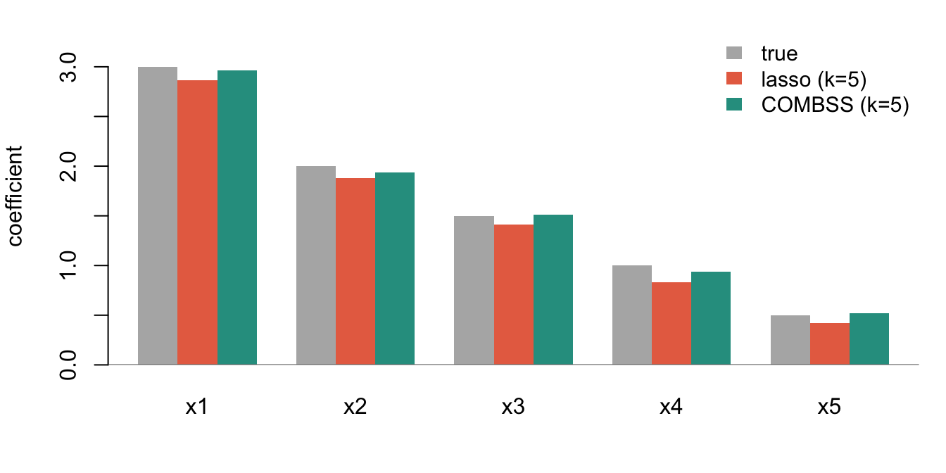
### 1. At a prescribed $k = 5$, how biased are the coefficients?

```{r}
#| label: combss-bias
#| echo: false
#| fig-width: 7
#| fig-height: 3.5
#| fig-cap: "Coefficients at $k=5$: True (grey), Lasso at the path-$\\lambda$ that gives 5 features and minimises training MSE (coral), and COMBSS (teal, OLS-refit on its $k=5$ subset). Squared $\\ell_2$ error to the truth across all 30 dimensions: **lasso 0.075, COMBSS 0.009** — ~8x smaller."

# Lasso at the lambda giving k=5 with smallest training MSE
idx5 <- which(nz == 5)
trn_mse_at5 <- sapply(idx5, function(i) {
  pred <- predict(fit_l, newx = X[itr, ], s = fit_l$lambda[i])
  mean((y[itr] - pred)^2)
})
lam5 <- fit_l$lambda[idx5[which.min(trn_mse_at5)]]
b_lasso5 <- as.numeric(coef(fit_l, s = lam5))[-1]

# COMBSS at k=5 with OLS refit
sel5 <- fit_c$subset_list[[5]]
ols  <- lm(y[itr] ~ X[itr, sel5])
b_combss5 <- rep(0, p)
b_combss5[sel5] <- coef(ols)[-1]

ix <- 1:5
mat <- t(cbind(true  = beta_true[ix],
               lasso = b_lasso5[ix],
               combss = b_combss5[ix]))
colnames(mat) <- paste0("x", ix)

par(mar = c(4, 4, 1, 1))
barplot(mat, beside = TRUE,
        col = c("grey70", "#e76f51", "#2a9d8f"),
        ylab = "coefficient",
        ylim = c(0, 3.4),
        border = NA)
abline(h = 0, col = "grey40")
legend("topright",
       legend = c("true", "lasso (k=5)", "COMBSS (k=5)"),
       fill = c("grey70", "#e76f51", "#2a9d8f"),
       border = NA, bty = "n", cex = 0.95)
```

COMBSS's recovered coefficients match the truth to within sampling noise. Lasso's are all visibly shrunken, even though both methods are looking at exactly five features.

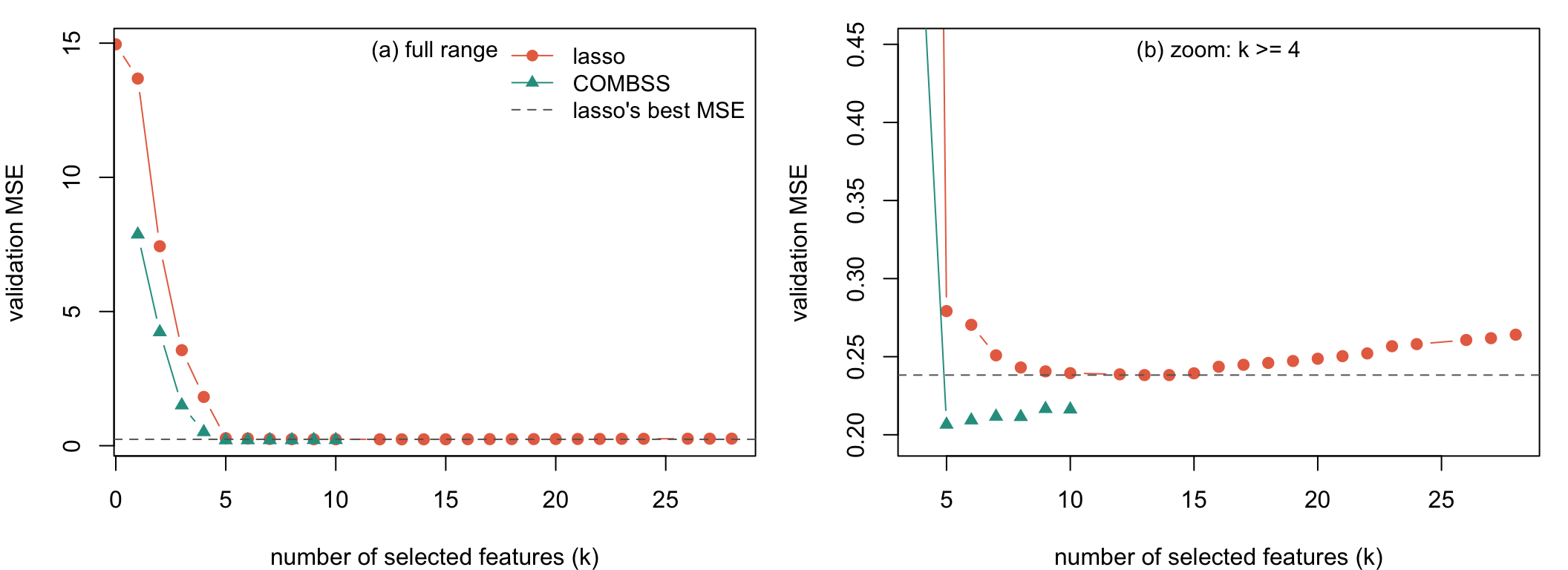
### 2. For the same validation loss, how many features does each method need?

```{r}
#| label: combss-mse-vs-k
#| echo: false
#| fig-width: 11
#| fig-height: 4
#| fig-cap: "**Left:** validation MSE as a function of the number of selected features (full range). **Right:** zoom into the region $k \\ge 4$ where the two methods plateau. The dashed line marks lasso's *best-ever* validation MSE. COMBSS at $k = 5$ already sits **below** that line — lasso cannot match COMBSS's $k=5$ performance at any model size."

# Validation MSE per unique k along the lasso path
ks_lasso <- sort(unique(nz))
val_mse_lasso <- sapply(ks_lasso, function(k) {
  i_k <- which(nz == k)
  trn <- sapply(i_k, function(i) {
    pred <- predict(fit_l, newx = X[itr, ], s = fit_l$lambda[i])
    mean((y[itr] - pred)^2)
  })
  pred_val <- predict(fit_l, newx = X[iva, ], s = fit_l$lambda[i_k[which.min(trn)]])
  mean((y[iva] - pred_val)^2)
})

# COMBSS val MSE per k from fit_c$mse_path
ks_combss <- seq_along(fit_c$mse_path)
val_mse_combss <- fit_c$mse_path

# Two-panel plot: full view + zoomed view
par(mfrow = c(1, 2), mar = c(4, 4, 1, 1))

# Panel 1: full view
plot(ks_lasso, val_mse_lasso, type = "b", pch = 19, col = "#e76f51",
     xlab = "number of selected features (k)",
     ylab = "validation MSE",
     ylim = range(c(val_mse_lasso, val_mse_combss)),
     xlim = c(1, max(c(ks_lasso, ks_combss))))
lines(ks_combss, val_mse_combss, type = "b", pch = 17, col = "#2a9d8f")
abline(h = min(val_mse_lasso), lty = 2, col = "grey40")
legend("topright",
       legend = c("lasso", "COMBSS", "lasso's best MSE"),
       col = c("#e76f51", "#2a9d8f", "grey40"),
       pch = c(19, 17, NA), lty = c(1, 1, 2),
       bty = "n", cex = 0.95)
mtext("(a) full range", side = 3, line = -1.2, cex = 0.95, adj = 0.5)

# Panel 2: zoomed in to k >= 4 where the plateau lives
keep_l <- ks_lasso >= 4
keep_c <- ks_combss >= 4
y_min <- min(val_mse_lasso[keep_l], val_mse_combss[keep_c]) - 0.01
y_max <- 0.45

plot(ks_lasso[keep_l], val_mse_lasso[keep_l], type = "b", pch = 19, col = "#e76f51",
     xlab = "number of selected features (k)",
     ylab = "validation MSE",
     ylim = c(y_min, y_max),
     xlim = c(4, max(ks_lasso)))
lines(ks_combss[keep_c], val_mse_combss[keep_c], type = "b", pch = 17, col = "#2a9d8f")
abline(h = min(val_mse_lasso), lty = 2, col = "grey40")
mtext("(b) zoom: k >= 4", side = 3, line = -1.2, cex = 0.95, adj = 0.5)

par(mfrow = c(1, 1))
```

At $k = 5$, COMBSS reaches a validation MSE that lasso cannot match at **any** model size — even with 22 features, lasso's MSE stays above COMBSS's value at $k = 5$.

## Preview of the rest of the talk

- **Methodology** — how the relaxation works, the Frank-Wolfe step, the curvature homotopy.
- **Demos** — five runnable demos showing the method in action.

::: {.page-nav}
[← Previous: Lasso](03-lasso.qmd)

[Next: Boolean relaxation →](../methodology/01-relaxation.qmd)
:::